New interface for selecting gene structure

Following previous post on new track selection interface, here I describe the similar change on gene structure selection function. Such function is used in Gene Set View and bigBed generator, and lets you decide which part of genes will be used.

Take custom gene set input for Gene Set View as example, open the control panel:

By default it shows "gene body" is in use. Click "change »" button, the gene structure selection panel will appear:

Check a radiobutton to select that gene part. If you need a custom region, check the "custom" option and the panel will become:

Same as before, you can press on the green/red sliders, slide them and select length for up/downstream flanking.

When you've done selecting, click anywhere else on page to dismiss the panel, and continue with usual process of running Gene Set View.

New interface about track selection

New user interface with somewhat radical change has been made for many browser components. I will use examples to introduce all of them.

First one will be heatmap track selection for statistical functions.

Heatmap track selection for pairwise comparison or hypothesis test

The pairwise comparison is to compare two groups of heatmap tracks. Open the pairwise comparison panel you will find two boxes indicating two group holders:

To assign track to group 1, click the "add »" button at top right corner of that box:

A new panel will be displayed with a list of currently displayed heatmap tracks in it. Click on one track name in this panel will assign that track into group 1. Blue background highlights that track as already selected:

Once you're done with the selection click anywhere else on the page to dismiss the track selection panel. Click X signs or buttons to remove track from this group.

The track selection for hypothesis test works in the same way. And don't forget you can do the same thing via right-click menus.

Track selection for correlation analysis

Go to the correlation panel, the interface of which has been stripped down to two buttons as the only operable components (compared with the cluttering old interface):

Click the first button, the heatmap selection panel will appear to let you select a track and run correlation against it:

Once a heatmap track has been selected, the panel will disappear and the correlation is turned on for that:

You can also choose a genomic feature track for correlation. Click that button for it:

This is a list of curated human genomic feature tracks available on the browser. As described before, genomic feature tracks are in separate groups and are arranged in parent-child style. In this panel, the left column is group names (Genes, Repeats, ...) and right is the collection of tracks belonging to this group. The arrow indicates there are children tracks associated with that track, and click it to reveal that:

So back to the correlation function, clicking on one of the genomic feature tracks will invoke correlation with that track (if the track is positional data like genes, correlation will be performed with its density data).

And as always, you can select a track for correlation via right-click menu options.



Managing genomic feature tracks

So here comes what I believe to be the most dramatic change: genomic feature track management component. Go to that panel:

A box is in the panel containing so called "your collection of genomic feature tracks". The browser provides many tracks but you might only be interested in a limited number of them. Having them neatly listed in this place would make management much easier compared with the old way.

Each entry in the list gently presents essential information about the track: name, type (bigBed), mode selector, removal button. Use the drop-down menu to change display mode:

And click the "Add more »" button opens the genomic feature track selection panel you've seen. You just take a look at the inventory, click on a track and it will be added to your list:

Other functions involving the use of track selection panel

1. Genomic juxtaposition

Selecting a track in this way will launch genomic juxtaposition for this track.

Notes:
1. you can only select genomic feature tracks with positional data, like genes, CpG islands, ... but not those with quantitative data, like GC content or conservation score.
2. Be aware about the amount of features displayed. If there's too many features displayed, running juxtaposition might take quite a bit of time (also depends on number of tracks are there in genome heatmap).




2. Gene Set sorting by track score

This option can be found after you run the Gene Set View. By choosing a heatmap track you can sort genes by their average score over that track.



Gene Plot

You will see this in the Gene Plot panel, where you will determine which quantitative track to be used for Gene Plot. You can either select any of the heatmap tracks, or select a genomic feature track with quantitative data (not the ones like gene model tracks).


*******

So now you might discover that buttons with » indicates it would launch a selector panel when pressed. Trust me I will stick to that.

These small revisions simplified the user interface of each function talked above, and made them consistent with each other, and got code complexity reduced. We hope you agree and would like to hear how you think.

Genome-wide statistics and visual display

Functionality of Bird's Eye View has been augmented, and now all types of quantitative tracks can be viewed through it. New additions are:

* pairwise comparison log-ratio
* hypothesis test P-values
* genomic feature density data


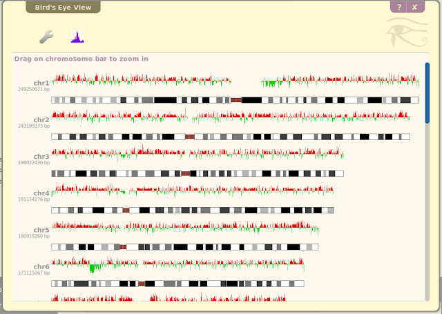
To view any of these data on a genome-wide scale, just right click on their track and select "Bird's eye view" option from the menu. The view will be generated in its own panel. It's that easy!


Genome-wide genomic feature density profile
In this example, right click on SINE element density track, the Bird's eye view option is available in menu:

Genome-wide SINE element density looks like this way:

Full-length demo on how to get genome-wide view of pairwise comparison

Take pairwise comparison as example. Suppose we want to compare two histone marks in H1 embryonic stem cell.

1. Go to the heatmap track selection panel at "Tracks" --> "Heatmap tracks". Make sure the panel is organized by "Sample" and "Epigenetic mark". By default the panel is fully expanded and is too big to look at. Click on the row/column header color blob to collapse the grid:

2. Click on relevant terms on row/column to reveal detail gradually, until we reach the terms we want. Finally it should look like (showing only part of the grid, with cursor upon H1-H3K4me3 tracks):

3. We need H3K4me3 and H3K4me1 data on H1 stem cell. First click "7/0" box, a new panel will appear in floating toolbox:

4. Press button and the 7 tracks will be placed in a new box and later we're going to add them for display.

5. Click "8/0" box in track selection grid and add H3K4me1-H1 tracks in same way, now we have 15 of them in "Heatmap tracks to be added" panel:

6. Press button , and all of them will be displayed in genome heatmap (the metadata heatmap has been configured to show only relevant entries):

7. At control panel, go to "Statistics & analysis" --> "Pairwise comparison". Now we're going to assign tracks to groups, H3K4me1 to one group, H3K4me3 to another group. A quick way to do this is via menu option on metadata heatmap:

8. Go back to pairwise comparison panel, having all tracks grouped, hit button , the log ratio track will be displayed:

9. Right click on log-ratio track, select "Bird's eye view" option:

And genome-wide comparison result is displayed:

10. If you click the "Vector" button with wiggle plot icon you will see all information about the pairwise comparison here in place:

So all participating tracks of pairwise comparison are available in the registry of Bird's Eye View. And row background color tells which group they belongs to, and the background color is derived from the bar color of pairwise track. If you change bar color, the group background color will change as well.


Genome-wide hypothesis test can be done with just the same way.
But running genome-wide hypothesis test is usually much slower than other birdeyeview operations. Please be patient and wait till result shows up.

New configuration methods for quantitative tracks

The Human Epigenome Browser specializes in visualizing quantitative data. But the solution was not good -- it only displayed tracks with positive values. It could be fine with slightly processed DNA sequencing data -- such as read density, peak calls, where all values are positive. But deeply processed data could have negative values. By fixing this problem of the Browser, a generic interface has been developed to allow user to control the style of all quantitative tracks in a consistent way. And the code got cleaned up as well.

By "quantitative track" I refer to a range of track types, so the configuration options described in this post applies to all of them, with different flavors:

• genome heatmap tracks
• numerical genomic feature tracks (e.g. GC percent, conservation scores)
• feature density of genomic feature tracks
• read density of custom BAM tracks
• pairwise comparison log-ratio tracks
• hypothesis test P-value tracks
• all the Bird's Eye View tracks

To begin with, right click on genome heatmap and select "Configure" option, following panel will show up in floating toolbox:

Let me explain things here, top to bottom:

Red and blue color blobs

These controls rendering color of the track, and positive/negative value colors will be determined separately. If the track is in heatmap mode, this color will be used for max/min data points. Any data in between will have lighter color. The baseline (at 0) color is always white. If the track is in wiggle style, the color is just bar color.

Click on the color blob, the color palette will be displayed near the cursor where you can pick up a color.

automatic/fixed/percentile scale

This option determines the scale. The first option "automatic scale" always set scale using max/min values. But if all the values are uniform (positive/negative), a 0-baseline will be enforced.

You can set fixed scale using second option, check it and the control panel will change a bit:

You can enter min/max values for the scale and press button to set that. Also in the color blobs two additional ones are shown, making things look complicated. They are colors for values beyond threshold, and this is actually very useful, as arbitrary combination of above/below threshold colors is made possible (which was impossible with the past design).

In the example below, values below max (which is set to be 30) will be bright red, and >= 30 it will be dark red. The tracks don't have negative value so blue color is not used:

The third option is actually what has been always used in the past: percentile threshold. Check it and the control panel will become:

There are still composite color blobs, means track values could be beyond threshold. The threshold now will be dynamically determined at a fixed percentile, and it is effective in getting rid of outlier values. Move the arrow above the ruler to select a percentile. Or you can click '>' '<' characters to increase/decrease percentile values (and it should work on your iPhone).

log transform

Will take logarithm of the track values. This is designed to be applied to ratio and P-value tracks. But you can apply it to wherever possible. Check the checkbox, options will appear for you to select base for the logarithm:

Above example shows applying log10 transform to MRE-Seq read density tracks (in heatmap style). Value below 1 will become negative and are plotted in blue.

Track height

Just the height of track. An implicit function is controlling heatmap/wiggle rendering style. If one track's height >= 20, it will be rendered as wiggle tracks, otherwise, it will be heatmap style.

apply to all tracks

This option is available if you are configuring heatmap tracks or bird's eye view tracks. If it is set to true, any subsequent change you make will be applied to all heatmap/birdeyeview tracks.

Following contents demonstrate how such configuration scheme applies to other types quantitative tracks, first of all, genomic feature density:

Genomic feature density 

Example shows configuring SINE element density data. As genomic feature density value can only be positive, only one color blob is displayed. And in order not to add mess, the log option is hidden. Just let me know if you're angry with it...

Quantitative decorative track

Example below is sequence conservation score track computed by PhyloP program. Both positive/negative color blobs, and log option are available for this type of tracks:

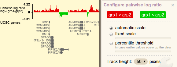
Pairwise comparison log-ratio

Red/blue color blobs controls bar color. Notice how the words change inside the blobs. As ratio values are always transformed by log2, logarithm option is not displayed.

Hypothesis test P-value

P-values are always between 0 and 1, and to emphasize those insanely small values, log10 transform is applied. Resulting values are all negative, and bars all point down... Don't scold me this is just things should be...

A horizontal line can appear in P-value track to indicate where cutoff value is. In the example it indicates the vertical position of 0.05. Bars stretching beyond the line are P-values lower than the cutoff, thus to be considered *significant*. Options are available in the panel to change cutoff value and line color, and the change will take place in a blink.

Bird's eye view tracks

All above track types can be viewed at the view angle of bird's eye, and can be configured in same manner. Following is such an example:

I'm glad to hear your opinion on these, just leave a comment!